How To : Apply Coning Compensation
Demonstrate coning compensation on integrated angular rate measurements [CIBS25].
 1import sys, os
 2
 3sys.path.insert(0, os.path.join("..", "..", ".."))
 4
 5import numpy as np
 6from scipy.interpolate import BPoly
 7
 8import matplotlib.pyplot as plt
 9
10# %matplotlib ipympl
11
12from functools import partial
13
14# Custom package for computing basis functions and derivatives
15from hitman.ode import butcher_tableaux, ButcherTableau
16from hitman.ode import rkmk_fixed_discrete
17from hitman.rotation import LieExponential as SO
18from hitman.plot import plot_hermite_spline
19from hitman.gyro import functional_factory
Measurement and Solution Functions
Consider the relationships
Our goal is to score methods for approximating change in attitude, \(\Delta \widetilde{R} \), from measurements \(\Delta \theta\). As a test case we define an attitude trajectory using a single polynomial function. We may choose to define either \(\omega\) or \(\phi\). The functional_factory() then generates measurement functional \( \Delta \theta \) and truth solution \( \Delta R \) from a single polynomial expression: either \(\omega\) or \(\phi\).
1# Benign trajectory
2A = np.array(
3 [
4 [1, 0, -1],
5 [4 / 3, 0, -4 / 3],
6 [11 / 6, 1 / 3, -11 / 3],
7 [5 / 2, 4 / 3, -4 - np.pi],
8 ]
9)
10is_omega = True
11
12# Generate random control points
13np.random.seed(0)
14A = np.random.randn(6, 3)
15is_omega = False
16
17# Form polynomial and required model functions
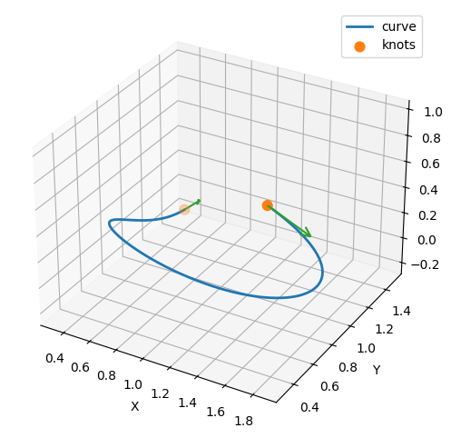
18f = BPoly(A[:, np.newaxis, :], [0.0, 1.0])
19_, _ = plot_hermite_spline(f, x=[0, 1])
20
21eval_delta_theta, eval_delta_R, eval_omega = functional_factory(f, is_omega)
Propagation Equations
Differential equations are typically expressed in terms of instantaneous rates. However, many gyroscopes provide integrate rate measurements. Since we have both instantaneous rates, eval_omega, and integrated rates, eval_delta_theta, we can contrast performance of state propagation algorithms from either measurement category.
Instantaneous Rate Propagation
Instantaneous rates can be propagated using the RKMK method [IMKNorsettZ00]. Different solver orders are utilized depending on which Butcher tableau specified. Note, the tableau determines the number of measurements required as well.
 1def rkmk(homega: np.ndarray, tableau: ButcherTableau) -> np.ndarray:
 2    """Solve attitude update from instantaneous rates
 3
 4    Args:
 5       homega: instantaneous rates, scaled by step size
 6       tableau: ButcherTableau specifying the RK method
 7
 8    Returns:
 9       Rotation matrix
10    """
11
12    # input checking
13    assert isinstance(tableau, ButcherTableau), "Input must be tableau"
14    N = np.unique(tableau.c).size
15    # size of homega must match tableau
16    assert (
17        homega.shape[0] == N
18    ), "For provided tableau, expecting %d samples of omega, received %d" % (
19        N,
20        homega.shape[0],
21    )
22
23    # apply rkmk algorithm and map to SO(3)
24    delta_phi = rkmk_fixed_discrete(homega, np.zeros_like(homega[0]), tableau)
25    return SO.exp(delta_phi)
Integrated Rate Propagation
Propagating integrated rate measurements requires models and approximations. One approach is to model the instantaneous rates as a curve fit to the integrated measurements. Generating samples of instantaneous rate enables use of generalized RK-style solvers.
 1def resample_delta_theta(
 2    delta_theta: np.ndarray, tau: float, sample_points=np.array([0, 0.5, 1])
 3):
 4    """Resample delta-theta measurements as polynomial fit of instantaneous rate"""
 5    if delta_theta.shape[0] == 1:
 6        homega_approx = delta_theta
 7    elif delta_theta.shape[0] == 2:
 8        A = np.array([[-0.5 * (tau**2), tau], [0.5 * (tau**2), tau]])
 9    elif delta_theta.shape[0] == 3:
10        A = np.array(
11            [
12                [(tau**3) / 3, -0.5 * (tau**2), tau],
13                [(tau**3) / 3, 0.5 * (tau**2), tau],
14                [7 * (tau**3) / 3, 1.5 * (tau**2), tau],
15            ]
16        )
17    else:
18        raise NotImplementedError(
19            "Requires one, two, or three delta-theta measurements"
20        )
21
22    if delta_theta.shape[0] > 1:
23        p = np.linalg.solve(A, delta_theta)
24        t_local = tau * sample_points
25        homega_approx = tau * np.vander(t_local, p.shape[0]) @ p
26
27    return homega_approx
Generalized solvers are computationally expensive. Instead of resampling instantaneous rates and applying generalized solvers, it is possible to approximate the solver solutions from integrated rate measurements directly [CIBS25]. Here we demonstrate approximations for 2 and 3 integrated rate measurements.
 1def SingleSpeed2(delta_theta):
 2    """Approximate delta-R from two delta-theta measurements"""
 3    assert delta_theta.shape[0] == 2, "Requires two delta-theta measurements"
 4    delta_phi = np.zeros_like(delta_theta[0])
 5    k = 1
 6    delta_phi += delta_theta[k] + np.cross(delta_theta[k - 1], delta_theta[k]) / 12
 7    return SO.exp(delta_phi)
 8
 9
10def SingleSpeed3(delta_theta):
11    """Approximate delta-R from three delta-theta measurements"""
12    assert delta_theta.shape[0] == 3, "Requires three delta-theta measurements"
13    delta_phi = np.zeros_like(delta_theta[0])
14    k = 1
15    delta_phi += (
16        delta_theta[k]
17        + (
18            np.cross(delta_theta[k + 1], delta_theta[k - 1])
19            + 13 * np.cross(delta_theta[k - 1] - delta_theta[k + 1], delta_theta[k])
20        )
21        / 12
22        / 24
23    )
24    return SO.exp(delta_phi)
Benchmark Algorithms
Define a dictionary of algorithms to contrast. For each algorithm, we indicate
func: solver functional to operate on the sampled ratesn_samples: number of samples required by the solverrate: whether the rate samples areinstantaneous, \(\omega\);integrated,\(\Delta \theta\); orresampledinstantaneous rates derived by curve fitting to integrated rates.
 1algorithm_dict = {
 2    "FwdElr_omega": {
 3        "func": partial(rkmk, tableau=butcher_tableaux["FwdElr"]),
 4        "n_samples": 1,
 5        "rate": "instantaneous",
 6    },
 7    "ExMid_omega": {
 8        "func": partial(rkmk, tableau=butcher_tableaux["ExpMid"]),
 9        "n_samples": 2,
10        "rate": "instantaneous",
11    },
12    "RK3_omega": {
13        "func": partial(rkmk, tableau=butcher_tableaux["RK3"]),
14        "n_samples": 3,
15        "rate": "instantaneous",
16    },
17    "RK4_omega": {
18        "func": partial(rkmk, tableau=butcher_tableaux["RK4"]),
19        "n_samples": 3,
20        "rate": "instantaneous",
21    },
22    "FwdElr_delta": {
23        "func": partial(rkmk, tableau=butcher_tableaux["FwdElr"]),
24        "n_samples": 1,
25        "rate": "resampled",
26    },
27    "ExMid_delta": {
28        "func": partial(rkmk, tableau=butcher_tableaux["ExpMid"]),
29        "n_samples": 2,
30        "rate": "resampled",
31    },
32    "RK3_delta": {
33        "func": partial(rkmk, tableau=butcher_tableaux["RK3"]),
34        "n_samples": 3,
35        "rate": "resampled",
36    },
37    "RK4_delta": {
38        "func": partial(rkmk, tableau=butcher_tableaux["RK4"]),
39        "n_samples": 3,
40        "rate": "resampled",
41    },
42    "SingleSpeed2": {
43        "func": SingleSpeed2,
44        "n_samples": 2,
45        "rate": "integrated",
46    },
47    "SingleSpeed3": {
48        "func": SingleSpeed3,
49        "n_samples": 3,
50        "rate": "integrated",
51    },
52}
Sample Trajectory
Define trajectory as a polynomial curve in \(\mathbb{R}\rightarrow \mathbb{R}^3\). The curve may represent \(\omega\) or \(\phi\).
Score algorithms and save results in :class:pandas.DataFrame.
 1import pandas as pd
 2import itertools
 3
 4# Increasing step sizes
 5tau_all = np.logspace(-6, -1, num=20)
 6
 7# Random sample points for trajectory
 8t_all = np.random.uniform(0.1, 0.9, 20)
 9
10# Generate all combinations of tau and t
11combinations = list(itertools.product(tau_all, t_all))
12
13# Create a DataFrame from the combinations
14df = pd.DataFrame(combinations, columns=["tau", "t"])
15
16# Iterate over each row in the DataFrame
17for index, row in df.iterrows():
18    tau = row["tau"]
19    t = row["t"]
20
21    # Generate instantaneous rate measurements
22    omega = np.array([eval_omega(t) for t in t + tau * np.arange(-1, 0.5, 0.5)])
23
24    # Generate sequential integrated rate measurements
25    delta_theta = np.vstack([eval_delta_theta(t + k * tau, tau) for k in range(-1, 2)])
26
27    # Define the truth eval_delta_R
28    Rstar = eval_delta_R(t, tau)
29    assert eval_omega([1, 1.5]).shape == (2, 3), "Wrong omega dims!"
30
31    # Benchmark each algorithm in the dictionary
32    for key, algorithm_data in algorithm_dict.items():
33        func = algorithm_data["func"]
34        n_samples = algorithm_data["n_samples"]
35        rate = algorithm_data["rate"]
36
37        if rate == "instantaneous":
38            # instantaneous rate measurements
39            #   * Note * RKMK requires measurements scaled by timestep!
40            dat = tau * np.atleast_2d(omega[0:n_samples, :])
41        elif rate == "integrated" or rate == "resampled":
42            dat = np.atleast_2d(delta_theta[0:n_samples, :])
43            if rate == "resampled":
44                # approximate h-omega by resampling
45                dat = resample_delta_theta(dat, tau)[0:n_samples, :]
46        else:
47            raise ValueError(f"Invalid rate: {rate}")
48
49        # propagate
50        Rhat = func(dat)
51        # score
52        err = np.linalg.norm(Rhat - Rstar)
53        # retain result
54        df.at[index, key] = err
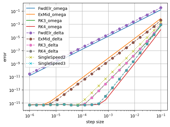
Plot Results
 1df_mean = df.groupby("tau").mean().reset_index()
 2
 3# get column names of df_mean (excluding 'tau')
 4column_names = df_mean.columns[2:].tolist()
 5
 6# plot loglog of df_mean using columns 1:-
 7for i, column in enumerate(column_names):
 8    if i < len(column_names) - 6:  # solid lines for first column
 9        linestyle = "-"
10        marker = None
11    elif i < len(column_names) - 2:  # solid lines for first column
12        linestyle = "--"
13        marker = "o"
14    else:
15        linestyle = ":"
16        marker = "x"
17
18    plt.loglog(
19        df_mean.iloc[:, 0],
20        df_mean[column],
21        linestyle=linestyle,
22        label=column,
23        marker=marker,
24    )
25# plt.ylim([1e-16, 1])
26plt.legend()
27plt.grid(True)
28plt.xlabel("step size")
29plt.ylabel("error")
30plt.show()